Artificial Neural Network (ANN) implementation on Breast Cancer Wisconsin Data Set using Python (keras)

Dataset

About Breast Cancer Wisconsin (Diagnostic) Data Set Features are computed from a digitized image of a fine needle aspirate (FNA) of a breast mass. They describe characteristics of the cell nuclei present in the image. n the 3-dimensional space is that described in: [K. P. Bennett and O. L. Mangasarian: “Robust Linear Programming Discrimination of Two Linearly Inseparable Sets”, Optimization Methods and Software 1, 1992, 23-34].

This database is also available through the UW CS ftp server: ftp ftp.cs.wisc.edu cd math-prog/cpo-dataset/machine-learn/WDBC/

Also can be found on UCI Machine Learning Repository: https://archive.ics.uci.edu/ml/datasets/Breast+Cancer+Wisconsin+%28Diagnostic%29

Attribute Information:

1) ID number 2) Diagnosis (M = malignant, B = benign) 3-32)

Ten real-valued features are computed for each cell nucleus:

a) radius (mean of distances from center to points on the perimeter) b) texture (standard deviation of gray-scale values) c) perimeter d) area e) smoothness (local variation in radius lengths) f) compactness (perimeter^2 / area - 1.0) g) concavity (severity of concave portions of the contour) h) concave points (number of concave portions of the contour) i) symmetry j) fractal dimension (“coastline approximation” - 1)

The mean, standard error and “worst” or largest (mean of the three largest values) of these features were computed for each image, resulting in 30 features. For instance, field 3 is Mean Radius, field 13 is Radius SE, field 23 is Worst Radius.

All feature values are recoded with four significant digits.

Missing attribute values: none

Class distribution: 357 benign, 212 malignant

Intro

To implement artificial neural network, I have used Keras which is a high-level Neural Networks API built on top of low-level neural networks APIs like Tensorflow and Theano. As it is high-level, many things are already taken care of therefore it is easy to work with and a great tool to start with.

Importing libraries

First of all, important useful libraries that need to preprocess and data and plot visuals

# Importing libraries
import pandas as pd
import numpy as np
import matplotlib.pyplot as plt
import seaborn as sns

Importing dataset and Preprocessing

After importing useful libraries I have imported Breast Cancer dataset, then first step is to separate features and labels from dataset then we will encode the categorical data, after that we have split entire dataset into two part: 70% is training data and 30% is test data. After that, we will scale the both training and testing datasets.

# Importing data
data = pd.read_csv('data.csv')
del data['Unnamed: 32']

#Feature and Label selection
X = data.iloc[:, 2:].values
y = data.iloc[:, 1].values

# Encoding categorical data
from sklearn.preprocessing import LabelEncoder
labelencoder_X_1 = LabelEncoder()
y = labelencoder_X_1.fit_transform(y)

# Splitting the dataset into the Training set and Test set (30 - 70)
from sklearn.model_selection import train_test_split
X_train, X_test, y_train, y_test = train_test_split(X, y, test_size = 0.3, random_state = 0)

#Feature Scaling
from sklearn.preprocessing import StandardScaler
sc = StandardScaler()
X_train = sc.fit_transform(X_train)
X_test = sc.transform(X_test)

Initialize the Artificial Neural Network (ANN)

The model needs to know what input shape it should expect. For this reason, the first layer in a Sequential model (and only the first, because following layers can do automatic shape inference) needs to receive information about its input shape. There are several possible ways to do this:

input_dim - number of columns of the dataset
output_dim - number of outputs to be fed to the next layer, if any
activation - activation function which is ReLU in this case
init - the way in which weights should be provided to an ANN

The ReLU function is f(x)=max(0,x). Usually this is applied element-wise to the output of some other function, such as a matrix-vector product. In MLP usages, rectifier units replace all other activation functions except perhaps the readout layer. One-way ReLUs improve neural networks is by speeding up training. The gradient computation is very simple (either 0 or 1 depending on the sign of x). Also, the computational step of a ReLU is easy: any negative elements are set to 0.0 – no exponentials, no multiplication or division operations.

import keras
from keras.models import Sequential
from keras.layers import Dense, Dropout

# Initialising the ANN
classifier = Sequential()

#===================================================================================================
# input_dim - number of columns of the dataset 
# 
# output_dim - number of outputs to be fed to the next layer, if any
# 
# activation - activation function which is ReLU in this case
# 
# init - the way in which weights should be provided to an ANN
#===================================================================================================

#----------------------------------------------------------------
#   INPUT LAYER
# input_dim: 30, output_dim: 16, init: uniform, activation:ReLu 
#
#   HIDDEN LAYER
# output_dim: 16, init: uniform, activation:ReLu 
#
#   OUTPUT LAYER
# output_dim:1, init: uniform, activation: sigmoid

#----------------------------------------------------------------

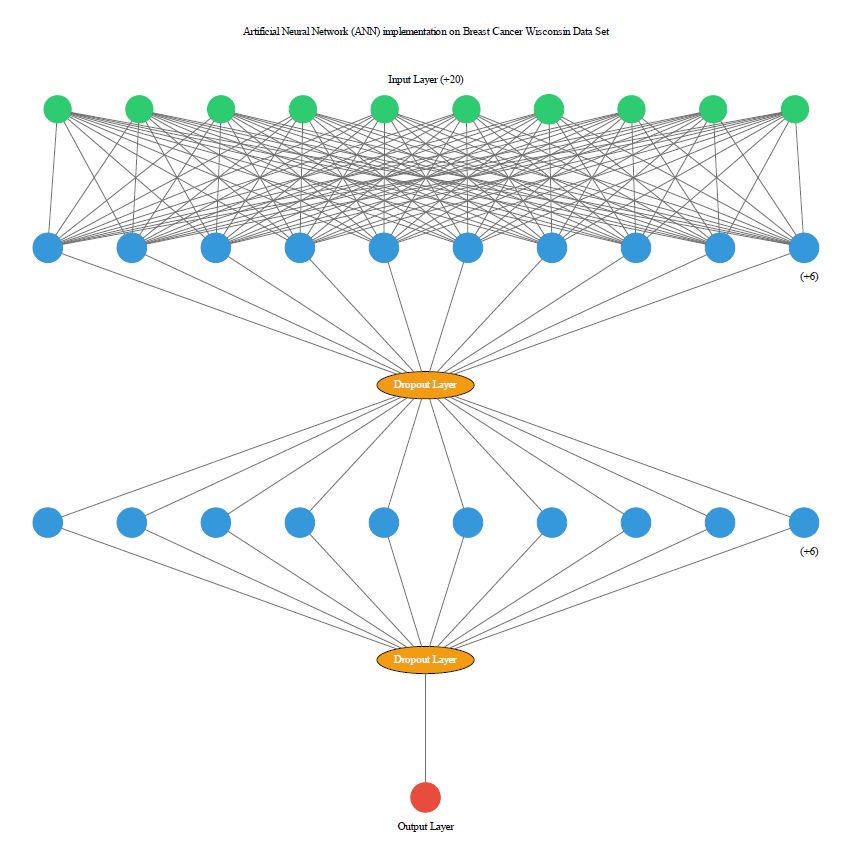
As we are using all feature so we have defined input layer with 30 perceptron along with 16 output dimensions after than we have used one hidden layer that consume output of input layer, both layers are using initiation values of ‘init’ and ‘ReLu’ activation function is being used at both layers, output layer is consuming output of hidden layer along with ‘sigmoid’ as activation function. The output layer is 1 as we want only 1 output from the final layer.

# Adding the input layer and the first hidden layer
classifier.add(Dense(output_dim=16, init='uniform', activation='relu', input_dim=30))
# Adding dropout to prevent overfitting
classifier.add(Dropout(p=0.1))


# Adding the second hidden layer
classifier.add(Dense(output_dim=16, init='uniform', activation='relu'))
# Adding dropout to prevent overfitting
classifier.add(Dropout(p=0.1))


# Adding the output layer (output_dim is 1 as we want only 1 output from the final layer.)
classifier.add(Dense(output_dim=1, init='uniform', activation='sigmoid'))

Optimizer

Just to improve the performance of model we have also applied some optimizer. Optimizer is chosen as ‘adam’ for gradient descent. ‘Binary_crossentrop’y is the loss function used. Cross-entropy loss, or log loss, measures the performance of a classification model whose output is a probability value between 0 and 1. Cross-entropy loss increases as the predicted probability diverges from the actual label. So, predicting a probability of .012 when the actual observation label is 1 would be bad and result in a high loss value. A perfect model would have a log loss of 0.

# Compiling the ANN
classifier.compile(optimizer='adam', loss='binary_crossentropy', metrics=['accuracy'])

Batch size defines number of samples that going to be propagated through the network. An Epoch is a complete pass through all the training data.

#---------------------------------------------------------
#   Epoch: 50
#---------------------------------------------------------

# Fitting the ANN to the Training set
classifier.fit(X_train, y_train, batch_size=100, nb_epoch=150)

Predicting the Test set results

As we have trained the model, so let predict the test using testing model

# Predicting the Test set results
y_pred = classifier.predict(X_test)
y_pred = (y_pred > 0.5)

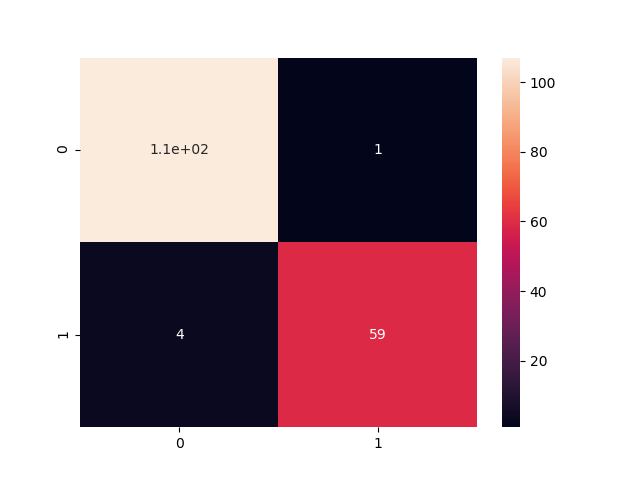
# Making the Confusion Matrix
from sklearn.metrics import confusion_matrix
cm = confusion_matrix(y_test, y_pred)


print("[Epoch:150] Our accuracy is {}%".format(((cm[0][0] + cm[1][1])/175)*100))

sns.heatmap(cm,annot=True)
plt.savefig('epoch150.png')

Accuracy

[Epoch:150] Our accuracy is 94.85714285714286%

Confusion Matrix

Visualization

Complete source avaiaable at https://github.com/MuhammadBilalYar/ann-on-breast-cancer-dataset